Jax Study
1. For loop
Jax has structure for for-loops using the jax.lax.fori_loop. The implementation executes the arguments to evaluate the following python code:
def fori_loop(lower, upper, body_fun, init_val):
    val = init_val
    for i in range(lower, upper):
        val = body_fun(i, val)
    return val
The value val should hold a fixed shape and dtype across all iterations. The key thing to note in this is that val can also just be a nested tuple/list/dict container with a fixed structure. There isn’t really a need to combine a fori_loop() with jit() since it compiles the function body_fun and hence jit becomes unnecessary for the function.
A quick way to use this is to have a step function that implements a single iteration of the intended loop and then use that as the argument for body_fun. For example:
import jax.numpy as jnp
from jax import lax

def forloop_example():
    result = jnp.zeros(10)
    def step(i, val):
        val = val.at[i].set(i)
        return val

    result = lax.fori_loop(0, len(result), step, result)
    return result

forloop_example()
No GPU/TPU found, falling back to CPU. (Set TF_CPP_MIN_LOG_LEVEL=0 and rerun for more info.)
Array([0., 1., 2., 3., 4., 5., 6., 7., 8., 9.], dtype=float32)
If we instead want to update multiple values in the for loop, we can return them as a tuple. For example
def forloop_example_multi():
    res1 = jnp.zeros(10)
    res2 = jnp.zeros(10)
    def step(i, val):
        res1, res2 = val
        res1 = res1.at[i].set(i)
        res2 = res2.at[i].set(len(res2)-i)
        return (res1, res2)

    res1, res2 = lax.fori_loop(0, len(res1), step, (res1, res2))
    return res1, res2

forloop_example_multi()
| Array | ((0 1 2 3 4 5 6 7 8 9) dtype=float32) | Array | ((10 9 8 7 6 5 4 3 2 1) dtype=float32) |
A thing to remember in this should be that all arrays can be updated only for a single number of iterations (as in a single for loop range).
2. Gradients
To calculate gradients of scalar functions in jax, we use the jax.grad() function. For example
from jax import grad, value_and_grad
def f(x):
    return x**2

value_and_grad(f)(3.0)
| Array | (9 dtype=float32 weaktype=True) | Array | (6 dtype=float32 weaktype=True) |
As we can see, using value_and_grad() we can get the value and gradient of a function at a value x. The gradient computation doesn’t support vectors as output of a function but the desired result can be achieved by using vmap().
value_and_grad(f)(jnp.arange(4.))
---------------------------------------------------------------------------
TypeError                                 Traceback (most recent call last)
Cell In[7], line 1
----> 1 value_and_grad(f)(jnp.arange(4.))

    [... skipping hidden 2 frame]

File ~/.local/share/virtualenvs/diff-mpm-zyodPdJl/lib/python3.10/site-packages/jax/_src/api.py:1274, in _check_scalar(x)
   1272 if isinstance(aval, ShapedArray):
   1273   if aval.shape != ():
-> 1274     raise TypeError(msg(f"had shape: {aval.shape}"))
   1275 else:
   1276   raise TypeError(msg(f"had abstract value {aval}"))

TypeError: Gradient only defined for scalar-output functions. Output had shape: (4,).
from jax import vmap
vmap(value_and_grad(f))(jnp.arange(4.))
| Array | ((0 1 4 9) dtype=float32) | Array | ((0 2 4 6) dtype=float32) |
Therefore, to vectorize gradient calculation on scalar output functions, vmap() can be used. But, this doesn’t help in calculating the gradients of functions that have a vector output.
def fvec(x):
    return jnp.array([x**2, x**3])

value_and_grad(fvec)(2.0)
---------------------------------------------------------------------------
TypeError                                 Traceback (most recent call last)
Cell In[11], line 4
      1 def fvec(x):
      2     return jnp.array([x**2, x**3])
----> 4 value_and_grad(fvec)(2.0)

    [... skipping hidden 2 frame]

File ~/.local/share/virtualenvs/diff-mpm-zyodPdJl/lib/python3.10/site-packages/jax/_src/api.py:1274, in _check_scalar(x)
   1272 if isinstance(aval, ShapedArray):
   1273   if aval.shape != ():
-> 1274     raise TypeError(msg(f"had shape: {aval.shape}"))
   1275 else:
   1276   raise TypeError(msg(f"had abstract value {aval}"))

TypeError: Gradient only defined for scalar-output functions. Output had shape: (2,).
To calculate these gradients, one way is to use jacobian().
from jax import jacobian

jacobian(fvec)(2.)
Array([ 4., 12.], dtype=float32, weak_type=True)
jacobian() can also accept vector inputs but it is important to understand the difference between using jacobian() with vector inputs and using vmap() with jacobian().
jacobian(fvec)(jnp.array([2., 3.]))
Array([[[ 4.,  0.],
        [ 0.,  6.]],

       [[12.,  0.],
        [ 0., 27.]]], dtype=float32)
vmap(jacobian(fvec))(jnp.array([2., 3.]))
Array([[ 4., 12.],
       [ 6., 27.]], dtype=float32)
As can be seen, when we use jacobian() with vector inputs, derivatives are calculated based on each of the input element, such that the original function is a function of n elements. On the other hand, if we just want the gradient of each return element of the function wrt to the single input element, we should use vmap(jacobian(f)) instead.
3. 1D Point Axial Vibration
3.1. Initialization
Computational Domain for this problem is set up as
L = 1                           # Domain size
nodes = jnp.array([0, L])       # Nodal coordinates
nnodes = len(nodes)             # Number of nodes
nelements = 1                   # Number of elements
nparticles = 1                  # Number of particles
el_length = L / nelements       # Element length
Material properties:
E = 4 * jnp.pi**2               # Young's modulus
rho = 1.                        # Density
Initial loading conditions:
v0 = 0.1                        # initial velocity
x_loc = 0.5                     # Location to get analytical solution
The material points in MPM keep track of position, mass, velocity, volume, momentum and stress. The material point is at the middle of the element and its volume is the size of the entire length of the bar.
x_p = 0.5 * el_length           # position of material point
mass_p = 1.                     # Mass of material point
vol_p = el_length / nparticles  # Volume
vel_p = v0                      # Initial velocity
stress_p = 0.                   # Stress
strain_p = 0.                   # Strain
momentum_p = mass_p * vel_p
3.1.1. Shape functions
For the shape function, we use a two-noded single element with linear elements.
def shape_fn(x):
    return 1 - abs(x - nodes)/L
For this shape function, we can write its derivative using jacobian(). The computed value can be confirmed by comparing to the analytical value of \(B(x) = [-1/L, 1/L]\).
vmap(jacobian(shape_fn))(jnp.array([0.1, 0.8]))
Array([[-1.,  1.],
       [-1.,  1.]], dtype=float32)
As we see, we get the correct value of the derivatives for 2 different values of x. Hence, we can define the derivative of the shape function as
def shape_fn_grad(x):
    return vmap(jacobian(shape_fn))(x)
3.2. Solution for a single step of time
During a single timestep, we perform the following actions
- Compute the nodal mass
- Compute nodal momentum
- Apply boundary conditions
- Compute external forces
- Compute internal forces
- Compute total unbalanced nodal forces
- Update nodal momentum
- Update particle position and velocities
- Update particle momentum
- Update nodal velocity
- Compute stress and strain
During this entire process, we want to store the evolution of velocity, position and energies with time.
t0, T, dt = 0, 10, 0.01
time = jnp.arange(t0, T, dt)
velocity = jnp.zeros(time.shape)
position = jnp.zeros(time.shape)
strain_energy = jnp.zeros(time.shape)
kinetic_energy = jnp.zeros(time.shape)

position = position.at[0].set(x_p)
velocity = velocity.at[0].set(vel_p)
Now, we will write a function that will perform one timestep update.
def step(i, kwargs):
    # Shape function and its derivative
    N = shape_fn(kwargs["position"][i-1])
    dN = jacobian(shape_fn)(kwargs["position"][i-1])

    # Nodal mass and momentum
    mass_n = N * kwargs["mass_p"]
    momentum_n = N * kwargs["momentum_p"]

    # Boundary conditions
    momentum_n = momentum_n.at[0].set(0)

    # External forces
    f_ext = jnp.array([0., 0.])

    # Internal forces
    f_int = -dN * kwargs["vol_p"] * kwargs["stress_p"]

    # Total nodal forces
    f_total = f_ext + f_int
    f_total = f_total.at[0].set(0)

    momentum_n += f_total * kwargs["dt"]

    # Update particle position and velocity
    vel_p = jnp.sum(kwargs["dt"] * N * f_total / mass_n) + kwargs["velocity"][i-1]
    pos_p = jnp.sum(kwargs["dt"] * N * momentum_n / mass_n) + kwargs["position"][i-1]

    # Update particle momentum
    kwargs["momentum_p"] = kwargs["mass_p"] * vel_p

    # Map nodal velocity
    vel_n = kwargs["mass_p"] * vel_p * jnp.divide(N, mass_n)
    vel_n = vel_n.at[0].set(0)

    # Strain rate at the particle
    strain_rate_p = jnp.dot(dN, vel_n)
    # Strain increment
    dstrain_p = strain_rate_p * dt
    # Strain
    kwargs["strain_p"] += dstrain_p
    kwargs["stress_p"] += kwargs["E"] * dstrain_p

    kwargs["velocity"] = kwargs["velocity"].at[i].set(vel_p)
    kwargs["position"] = kwargs["position"].at[i].set(pos_p)

    # Compute and store strain energy
    se = 0.5 * kwargs["stress_p"] * kwargs["strain_p"] * kwargs["vol_p"]
    kwargs["strain_energy"] = kwargs["strain_energy"].at[i].set(se)

    # Compute and store kinetic energy
    ke = 0.5 * vel_p**2 * kwargs["mass_p"]
    kwargs["kinetic_energy"] = kwargs["kinetic_energy"].at[i].set(ke)
    return kwargs
We can now use this function in the jax.lax.fori_loop() function to run the iterations.
kwargs = {
    "mass_p": mass_p,
    "vol_p": vol_p,
    "stress_p": stress_p,
    "strain_p": strain_p,
    "momentum_p": momentum_p,
    "velocity": velocity,
    "position": position,
    "strain_energy": strain_energy,
    "kinetic_energy": kinetic_energy,
    "E": E,
    "dt": dt,
}
result = lax.fori_loop(1, len(time), step, kwargs)
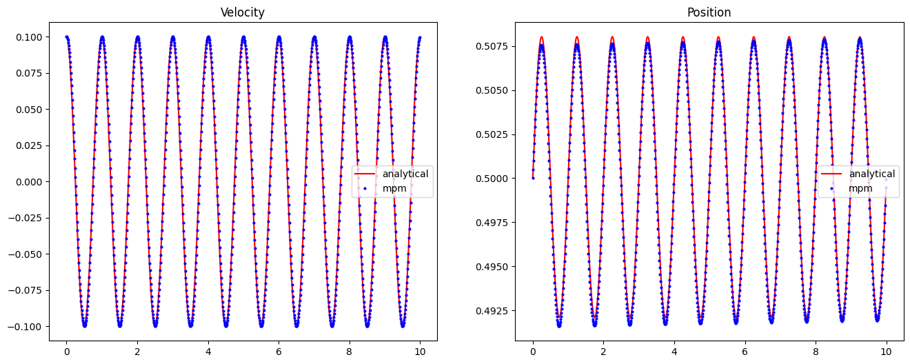
We can compare this result with the analytical solution which can be evaluated as follows:
def analytical_vibration(E, rho, v0, x_loc, duration, dt, L):
    omega = 1 / L * jnp.sqrt(E / rho)
    t = jnp.arange(0, duration, dt)
    v = v0 * jnp.cos(omega * t)
    x = x_loc * jnp.exp(v0 / (L * omega) * jnp.sin(omega * t))
    return x, v


xa, va = analytical_vibration(E, rho, v0, x_loc, T, dt, L)
import matplotlib.pyplot as plt

fig, ax = plt.subplots(1, 2, figsize=(16, 6))
ax[0].plot(time, va, "r", label="analytical")
ax[0].plot(time, result["velocity"], "ob", markersize=2, label="mpm")
ax[0].legend()
ax[0].set_title("Velocity")

ax[1].plot(time, xa, "r", label="analytical")
ax[1].plot(time, result["position"], "ob", markersize=2, label="mpm")
ax[1].legend()
ax[1].set_title("Position")
fig.savefig("../assets/mpm_plots.png")